QK Box 10.6

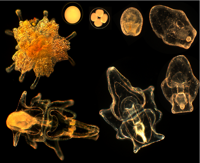
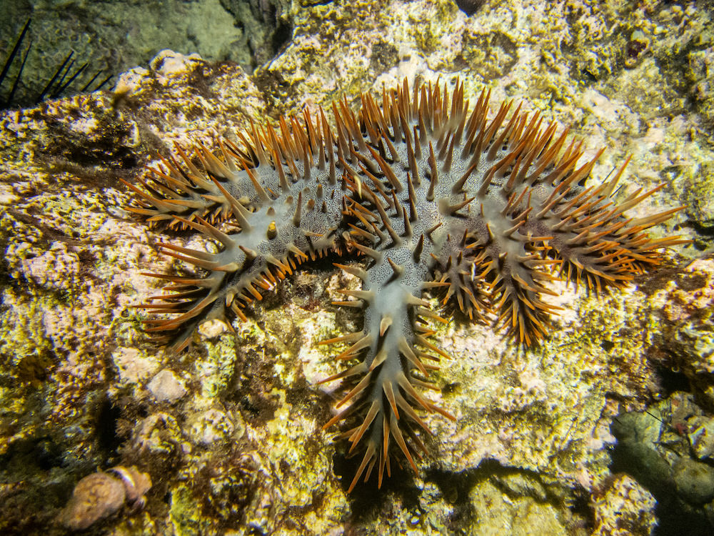
Caballes et al. (2016) examined the effects of maternal nutrition (three treatments: starved or fed one of two coral genera: Acropora or Porites) on the larval biology of crown-of-thorns seastars. There were three female seastars nested within each treatment, 50 larvae reared from each female were placed into each of three glass culture jars and the lengths of ten larvae from each jar after four days were measured after 4 days. This fully balanced design has maternal nutrition as a fixed factor with three random levels of nesting: females within nutrition treatment, jars within females and individual larvae within jars.

Crown of thorns seastar, Acanthaster planci. Mick Keough, CC BY 4.0

Larval cycle of crown-of-thorns. AIMS, CC BY 4.0

The paper is here

Caballes, C. F., Pratchett, M. S., Kerr, A. M. & Rivera-Posada, J. A. (2016). The role of maternal nutrition on oocyte size and quality, with respect to early larval development in the coral-eating starfish, Acanthaster planci. PLoS One, 11, e0158007.

Preliminaries

Packages:

library(tidyverse)
source("R/set_ggplot_theme.R")
library(broom)
library(Rmisc)
library(car)
library(lme4)
library(lmerTest)
library(nlme)
library(VCA)
library(afex)

Data:

caballes_length <- read.csv("data/caballes_length.csv")

set_sum_contrasts()

Make female and jar factors

caballes_length$female <- factor(caballes_length$female)
caballes_length$jar <- factor(caballes_length$jar)

Reorder nutrition treatments so starved is first for default lm contrasts

caballes_length$diet <- factor(caballes_length$diet, levels = c("starved","aa","pr"))
levels(caballes_length$diet)

[1] "starved" "aa"      "pr"     

Visualize data

caballes_length %>% 
  ggplot(aes(jar, length, color = female)) + 
  geom_point(alpha = 0.5) +
  facet_wrap(~ diet, scales = "free_x")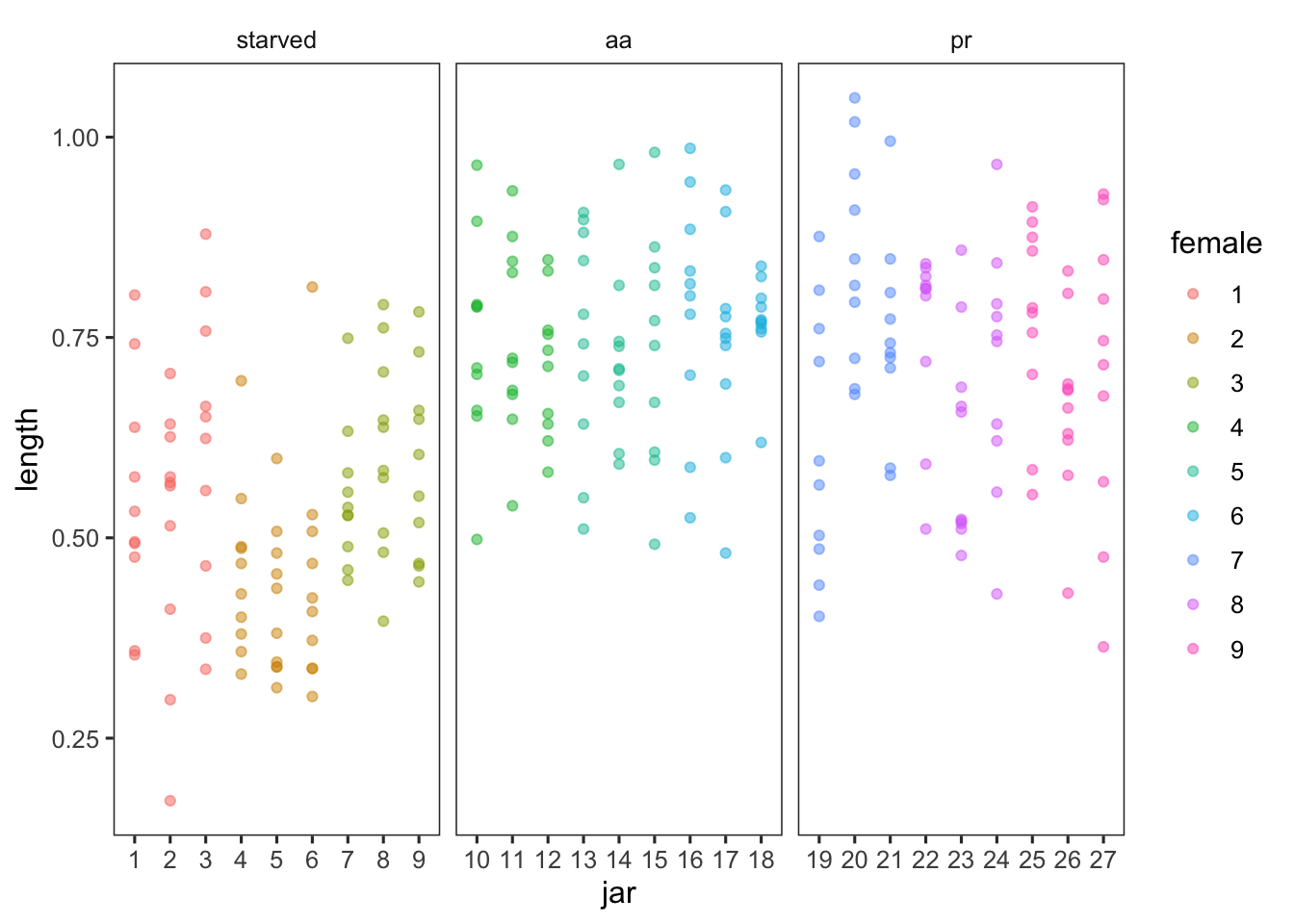

Run model

Note: can’t get the aov commands to work for 3 level nested design

caballes.aov <- aov(length~diet+Error(female/jar), caballes_length)

Fit as lm using OLS estimation

caballes.lm <- lm(length ~ diet/female/jar, caballes_length)
anova(caballes.lm)

Analysis of Variance Table

Response: length
                 Df Sum Sq Mean Sq F value    Pr(>F)    
diet              2 2.5334 1.26668 72.1624 < 2.2e-16 ***
diet:female       6 0.3735 0.06224  3.5460  0.002199 ** 
diet:female:jar  18 0.5265 0.02925  1.6664  0.045989 *  
Residuals       243 4.2654 0.01755                      
---
Signif. codes:  0 '***' 0.001 '**' 0.01 '*' 0.05 '.' 0.1 ' ' 1

Check diagnostics and lm output (not shown):

plot(caballes.lm)
summary(caballes.lm)

Get F and P values using correct denominators

#Diet F
f <- 1.26668/0.06224
pf(f, df1 = 2, df2 = 6, lower.tail = FALSE)

[1] 0.002120396

#Females F
f <- 0.06224/0.02925
pf(f, df1 = 6, df2 = 18, lower.tail = FALSE)

[1] 0.100229

#Jars F
f <- 0.02925/0.01755
pf(f, df1 = 18, df2 = 243, lower.tail = FALSE)

[1] 0.04594475

Variance components from VCA

caballes.vca <- anovaMM(length ~ diet/(female)/(jar), caballes_length)
caballes.vca
VCAinference(caballes.vca, alpha = 0.05, VarVC = TRUE, ci.method = "satterthwaite")

Fit mixed effects model using REML/ML

caballes.lmer <- lmer(length ~ diet + (1|female/jar), caballes_length)
summary(caballes.lmer)

Linear mixed model fit by REML. t-tests use Satterthwaite's method [
lmerModLmerTest]
Formula: length ~ diet + (1 | female/jar)
   Data: caballes_length

REML criterion at convergence: -289.2

Scaled residuals: 
     Min       1Q   Median       3Q      Max 
-2.69014 -0.69659  0.01388  0.64143  2.59374 

Random effects:
 Groups     Name        Variance Std.Dev.
 jar:female (Intercept) 0.00117  0.03420 
 female     (Intercept) 0.00110  0.03316 
 Residual               0.01755  0.13249 
Number of obs: 270, groups:  jar:female, 27; female, 9

Fixed effects:
            Estimate Std. Error       df t value Pr(>|t|)    
(Intercept)  0.66279    0.01518  5.99986  43.652 9.68e-09 ***
diet1       -0.13588    0.02147  5.99986  -6.328 0.000728 ***
diet2        0.08301    0.02147  5.99986   3.866 0.008306 ** 
---
Signif. codes:  0 '***' 0.001 '**' 0.01 '*' 0.05 '.' 0.1 ' ' 1

Correlation of Fixed Effects:
      (Intr) diet1 
diet1  0.000       
diet2  0.000 -0.500

Get F-ratio for diet test using lmerTest

anova(caballes.lmer, ddf = "Kenward-Roger")

Type III Analysis of Variance Table with Kenward-Roger's method
      Sum Sq Mean Sq NumDF DenDF F value   Pr(>F)   
diet 0.71442 0.35721     2     6   20.35 0.002121 **
---
Signif. codes:  0 '***' 0.001 '**' 0.01 '*' 0.05 '.' 0.1 ' ' 1

CI on variance components (remembering to square CIs from lmer which are in SD units)

caballes.ci <- confint.merMod(caballes.lmer)
caballes.vc <- (caballes.ci)^2
print(caballes.vc)

                  2.5 %      97.5 %
.sig01      0.000000000 0.004051007
.sig02      0.000000000 0.003177589
.sigma      0.014769187 0.021083239
(Intercept) 0.404053917 0.475997080
diet1       0.030364676 0.009506432
diet2       0.001992217 0.014735036

Simplify dataset by averaging across larvae within a jar

d <- caballes_length %>% 
  group_by(diet, female, jar) %>%
  dplyr::summarise(mean = mean(length), 
            sd = sd(length), 
            n = n(), 
            se = sd / sqrt(n)) %>% 
  ungroup()

d %>% 
  ggplot(aes(female, mean)) + 
  geom_point(alpha = 0.5) +
  facet_wrap(~ diet, scales = "free_x") + 
  labs(y = "Mean length (mm)")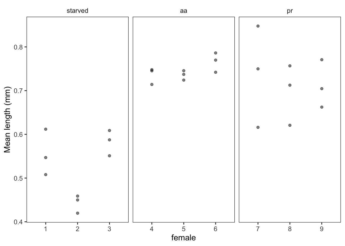

Fit nested ANOVA with OLS

Female is nested within treatment:

d_aov <- aov(mean~diet+Error(female), d)
summary(d_aov)

Error: female
          Df  Sum Sq Mean Sq F value  Pr(>F)   
diet       2 0.25334 0.12667   20.35 0.00212 **
Residuals  6 0.03735 0.00622                   
---
Signif. codes:  0 '***' 0.001 '**' 0.01 '*' 0.05 '.' 0.1 ' ' 1

Error: Within
          Df  Sum Sq  Mean Sq F value Pr(>F)
Residuals 18 0.05265 0.002925               

m1 <- lm(mean ~ diet / female, d)
anova(m1)

Analysis of Variance Table

Response: mean
            Df   Sum Sq  Mean Sq F value    Pr(>F)    
diet         2 0.253336 0.126668 43.3035 1.323e-07 ***
diet:female  6 0.037346 0.006224  2.1279    0.1002    
Residuals   18 0.052652 0.002925                      
---
Signif. codes:  0 '***' 0.001 '**' 0.01 '*' 0.05 '.' 0.1 ' ' 1

Get F and P values using correct denominators. Note that I’m using broom:tidy to tidy the anova output, and lead() to calculate the new_F and new_P. This avoids extracting statistic (F-value) and df into new objects, or hard-coding the calculations.

tidy(anova(m1)) %>% 
  mutate(new_F = meansq / lead(meansq), 
         new_P = pf(new_F, df1 = df, df2 = lead(df), lower.tail = FALSE)) %>% 
  kable(digits = 3)

term	df	sumsq	meansq	statistic	p.value	new_F	new_P
diet	2	0.253	0.127	43.303	0.0	20.351	0.002
diet:female	6	0.037	0.006	2.128	0.1	2.128	0.100
Residuals	18	0.053	0.003	NA	NA	NA	NA

Fit mixed effects model using REML/ML

m2 <- lmer(mean ~ diet + (1|female), d)
summary(m2)

Linear mixed model fit by REML. t-tests use Satterthwaite's method [
lmerModLmerTest]
Formula: mean ~ diet + (1 | female)
   Data: d

REML criterion at convergence: -58.6

Scaled residuals: 
     Min       1Q   Median       3Q      Max 
-2.05994 -0.46141  0.08908  0.48149  2.22410 

Random effects:
 Groups   Name        Variance Std.Dev.
 female   (Intercept) 0.001100 0.03316 
 Residual             0.002925 0.05408 
Number of obs: 27, groups:  female, 9

Fixed effects:
            Estimate Std. Error       df t value Pr(>|t|)    
(Intercept)  0.66279    0.01518  6.00000  43.653 9.68e-09 ***
diet1       -0.13588    0.02147  6.00000  -6.328 0.000728 ***
diet2        0.08301    0.02147  6.00000   3.866 0.008305 ** 
---
Signif. codes:  0 '***' 0.001 '**' 0.01 '*' 0.05 '.' 0.1 ' ' 1

Correlation of Fixed Effects:
      (Intr) diet1 
diet1  0.000       
diet2  0.000 -0.500

anova(m2, ddf = "Kenward-Roger")

Type III Analysis of Variance Table with Kenward-Roger's method
      Sum Sq  Mean Sq NumDF DenDF F value   Pr(>F)   
diet 0.11906 0.059528     2     6   20.35 0.002121 **
---
Signif. codes:  0 '***' 0.001 '**' 0.01 '*' 0.05 '.' 0.1 ' ' 1